Precipitation Simulation of Ni-14Al (at%) Alloy
Purpose: Learn to perform a precipitation simulation of a binary alloy. In this example, precipitation simulation will be performed for Ni-14Al alloy during isothermal ageing at 550 °C, and experimental data will be added to the plots
Module: PanEvolution
Thermodynamic and Mobility Database:AlNi_Prep.tdb
Kinetic Parameters Database: Ni-14Al_Precipitation.kdb
Batch file: Example_#3.1.pbfx
Calculation Procedures:
-
Create a workspace and select the PanEvolution module following Pandat User's Guide: Workspace;
-
Load AlNi_Prep.tdb following the procedure in Pandat User's Guide: Load Database ;
-
Click on PanEvolution/PanPrecipitation on the menu bar and select "Load KDB or EKDB", then select the Ni-14Al_Precipitation.kdb, a dialog will pop out as shown in Figure 1. This dialog shows the key information stored in the Ni-14Al_Precipitation.kdb, i.e, the matrix phase is Fcc, and the precipitate phase is L12_FCC;
-
Click menu "File → Open File" to open the Ni-14Al_Precipitation.kdb. As shown in Figure 2, in addition to the matrix phase and precipitate phase, other parameters, such as, molar volume and interfacial energy are also defined in this file. Details on these parameters can be found in Pandat User's Guide: The Kinetic Parameters Database (KDB file) Syntax and Examples;
-
Click on PanEvolution/PanPrecipitation on the menu bar and click "Precipitation Simulation". A dialog will pop out as shown in Figure 1, set up the alloy chemistry on the left and the heat treatment condition on the right. In this setting, an isothermal ageing is performed at 550 °C assuming the initial state is pure Fcc phase; Add Intermediate PSD outputs at 1 hour, 10 hours and 50 hours.
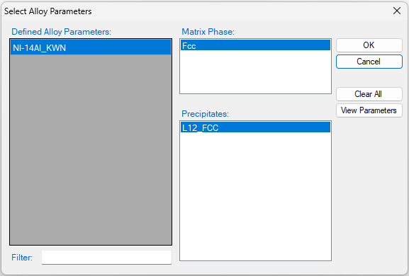
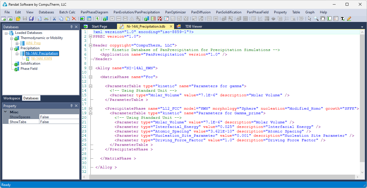

Figure 3: Setup the alloy chemistry (Ni-14 at%Al) and heat treatment condition (isothermal ageing at 550 °C) for the simulation
Post Calculation Operation:
-
Right click the Default graph and rename it as Vf;
-
Create a new table as shown in Figure 4. A new table with two columns will be created with the first time in hour and the second size of L12_FCC in nanometer. Create a plot from this table and rename it as Size;
-
Create a new table as shown in Figure 5. A new table with two columns will be created with the first log(time in minute) and the second the number density of L12_FCC in cm3. Create a plot from this table and rename it as nd;
-
Import a table from a file as shown in Figure 6, and select Ni-14Al_Exp.dat;
-
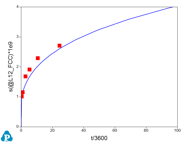
Open the Size graph, single click the Ni-14Al_Exp table and drag in the t(hr) as x-axis, press Ctrl and drag in the radius(nm) as y-axis. In the Property window set the "Plot Type" as Point, the plot with experimental data point is shown in Figure 7;
-
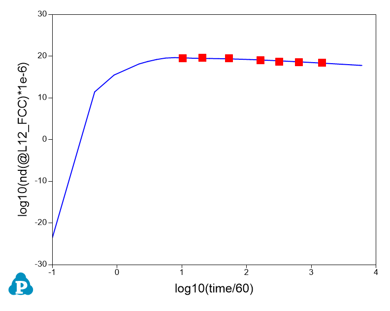
Open the nd graph and add the experimental data on it as shown in Figure 8;
-
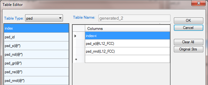
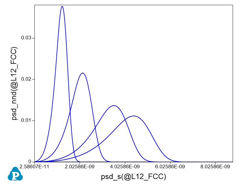
Create a new table as shown in Figure Figure 9, select psd as the Table Type; select the psd_s(L12_FCC) and the psd_nnd(L12_FCC) two columns to create a new plot as shown in Figure 10;
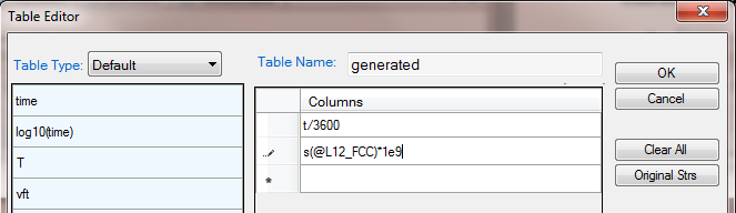
Figure 4: Create a new table with two columns with the first column time (hour) and the second column the precipitate size (nm)
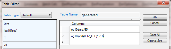
Figure 5: Create a new table with two columns with the first column log(time) and the second the number density of the precipitate per cm^3


Information obtained from this calculation:
-
It is common practice to plot the experimental data on the calculated diagram. When doing so, it is important to make unit consistency between the experimental data and the calculated property. In Pandat™ calculation, international standard unit is used, i.e., second for time, meter for length and cube meter for volume, and so on;
-
Particle number density counts the number of particles in a unit volume. Default output from Pandat is number per m3, it was converted to number per cm3 in Figure 8;
-
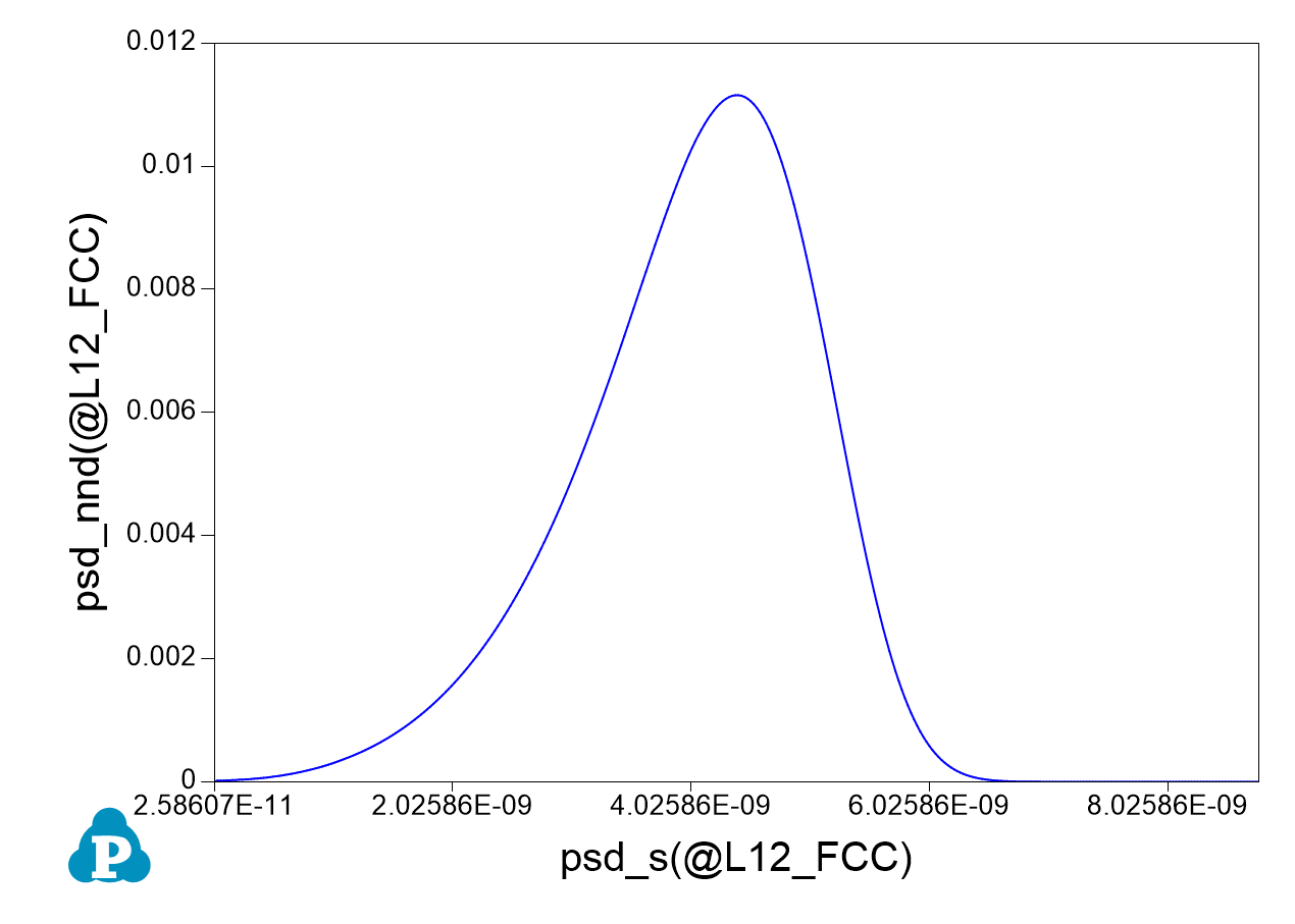
The psd_nnd(L12_FCC) in Figure 10 is normalized number density, which equals to the particle numbers of each size class divided by the total particle numbers;
-
Figure 10 shows four distribution curves at four different times. The sharp one is at early nucleation stage which shows small particle size and high number density, the flat one shows the particle size distribution as final time (100 hours in this simulation). The corresponding time of each distribution can be found in the table. When create the table, simply put this time information in the table as shown in Figure 11;
-
To only plot the particle size distribution curve at one time, set the inde x=1, or 2 ... or i. index=i means the final distribution. Figure 12 shows the table created for the final size distribution and Figure 13 shows the distribution curve.